
Contents:
Data Quality
4.1 Normality
4.2 Outlier
4.3 Correlation
4.4 Regression
5. Basic assumptions
5.1. Classification theory (false positive and negative)
5.1.1. Variance, ANOVA
5.1.2 MANOVA
What is Discriminant function analysis ?
A statistical discrimination of classification problem consists in assigning or classifying an individual or group of individuals to one of several known or unknown alternative populations on the basis of several measurements on the individual and samples from the unknown populations. For example, a linear combination of the measurements, called the linear discriminator or discriminant function, is constructed on the basis of its value the individual is assigned to one or the other of two populations.
Discriminant function analysis is a
statistical analysis to predict a
categorical dependent variable (called a grouping variable) by one or more
continuous or binary independent variables (called predictor variables).The
main purpose of a discriminant function analysis is to predict
group membership based on a linear combination of the interval variables. The
procedure begins with a set of observations where both group membership and the
values of the interval variables are known. DFA is different from MDA.
MDA is a statistical technique used to reduce the differences between variables
in order to classify them into a set number of broad groups. Discriminant function analysis is reversed of multivariate analysis of
variance (MANOVA). In MANOVA, the independent variables are the groups and the
dependent variables are the predictors.
Assumptions
Dependent and Independent Variables
- The dependent variable should be categorized
by m (at least 2) text values (e.g.: 1-good student, 2-bad student; or
1-prominent student, 2-average, 3-bad student). If the dependent variable
is not categorized, but its scale of measurement is interval or ratio
scale, then we should categorize it first. For instance the average
scholastic record is measured by ratio scale, however, if we categorize
them as students with average scholastic record over 4.1 are considered
good, between 2.5 and 4.0 they are average, and below 2.5 the students are
bad, this variable will fulfill the requirements of discriminant analysis.
- However, we can ask: why did students over 4.1
are known as good student? Why 2.5 is the bound to consider the students
bad? Due to this subjective categorization the analysis can be biased, or
the correlation coefficients can be under- or overestimated. To remedy
this, try to create similar size of categories. It is easier by creating
graph about the distribution of dependent variables or relying on prior
information. Statistical software, which contains discriminant analysis,
such as SPSS, has an option, which recodes variables. However, it is more
significant using already categorical variables, because in other case, we
will lose some information. In case of non-categorical variables it would
be better to use regression analysis instead of discriminant analysis.
- Independent variables should be metric. We do
not have to standardize variables for discriminant analysis, because the
unit of measures does not have decisive influence. Therefore, any metric
variable can be selected for independent variable. If we have a sufficient
number of quantitative variables, we can build dichotomies or ordinal
scaled variables with at least 5 categories in the model (Sajtos – Mitev,
2007).
Normality
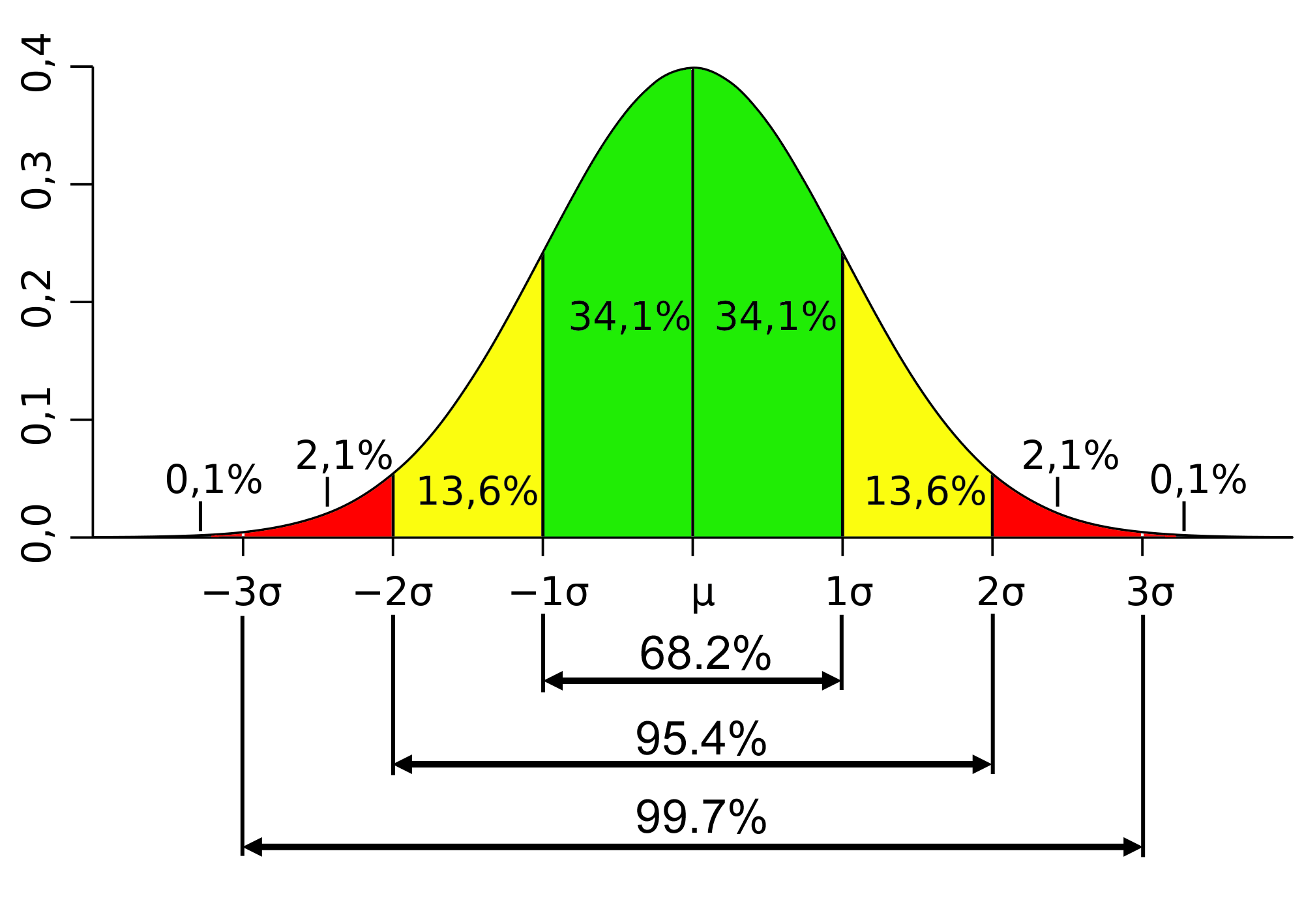
http://www.muelaner.com/wp-content/uploads/2013/07/Standard_deviation_diagram.png
- · The mean, median, and mode of a normal distribution are equal. The area under the normal curve is equal to 1.0. Normal distributions are denser in the center and less dense in the tails. Normal distributions are defined by two parameters, the mean (μ) and the standard deviation (σ).
- · The Standard Normal curve, shown here, has mean 0 and standard deviation 1. If a dataset follows a normal distribution, then about 68% of the observations will fall within of the mean , which in this case is with the interval (-1,1).
- · As far as I understand, attention should be paid to the normal distribution of variables along with the size.
OUTLIER
- It refers to a person or thing situated away or detached from the main body or system.In statistics, an outlier is an observation point that is distant from other observations.
- An outlier may be due to
- variability in the measurement or
- it may indicate experimental error; the latter are sometimes excluded from the data set.
- sampling error
- Measurement errors can be divided into two components: random error and systematic error
- Random errors are errors in measurement that lead to measurable values being inconsistent when repeated measurements of a constant attribute or quantity are taken.
- Systematic errors are errors that are not determined by chance but are introduced by an inaccuracy (involving either the observation or measurement process) inherent to the system.
- Systematic error may also refer to an error with a nonzero mean, the effect of which is not reduced when observations are averaged.
- Sources of systematic error may be
- imperfect calibration of measurement instruments (zero error)
- changes in the environment which interfere with the measurement process
- imperfect methods of observation
- Random errors may ocuur from non-sampling errors ( the errors are not due to sampling)
- Non-sampling errors in survey estimates can arise from:
- Coverage errors, such as failure to accurately represent all population units in the sample, or the inability to obtain information about all sample cases;
- Response errors by respondents due for example to definitional differences, misunderstandings, or deliberate misreporting;
- Mistakes in recording the data or coding it to standard classifications;
- Other errors of collection, nonresponse, processing, or imputation of values for missing or inconsistent data.
Measurement error can cause statistical error.Statistical error is the amount by which an observation differs from its expected value, the latter being based on the whole population from which the statistical unit was chosen randomly. For example, if the mean height in a population of 21-year-old men is 1.75 meters, and one randomly chosen man is 1.80 meters tall, then the "error" is 0.05 meters; if the randomly chosen man is 1.70 meters tall, then the "error" is −0.05 meters. The expected value, being the mean of the entire population, is typically unobservable, and hence the statistical error cannot be observed either.
Other assumptions are (Sajtos – Mitev, 2007):
|
The assumptions of discriminant analysis are the same
as those for MANOVA. The analysis is quite
sensitive to outliers and the size of the smallest group must be larger than
the number of predictor variables. Multivariate normality: Independent
variables are normal for each level of the grouping variable.
Normality:
a ratio between +1 and −1 calculated so as to represent the linear interdependence of two variables or sets of data.
Pearson Product-Moment Correlation
What does this test do?
The Pearson product-moment correlation coefficient (or Pearson correlation coefficient, for short) is a measure of the strength of a linear association between two variables and is denoted by r. Basically, a Pearson product-moment correlation attempts to draw a line of best fit through the data of two variables, and the Pearson correlation coefficient, r, indicates how far away all these data points are to this line of best fit (i.e., how well the data points fit this new model/line of best fit).
What values can the Pearson correlation coefficient take?
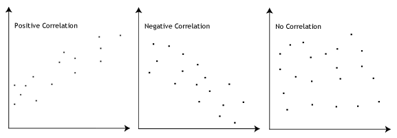
The Pearson correlation coefficient, r, can take a range of values from +1 to -1. A value of 0 indicates that there is no association between the two variables. A value greater than 0 indicates a positive association; that is, as the value of one variable increases, so does the value of the other variable. A value less than 0 indicates a negative association; that is, as the value of one variable increases, the value of the other variable decreases. This is shown in the diagram below:
How can we determine the strength of association based on the Pearson correlation coefficient?
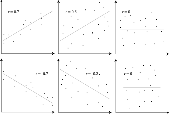
The stronger the association of the two variables, the closer the Pearson correlation coefficient, r, will be to either +1 or -1 depending on whether the relationship is positive or negative, respectively. Achieving a value of +1 or -1 means that all your data points are included on the line of best fit – there are no data points that show any variation away from this line. Values for r between +1 and -1 (for example, r = 0.8 or -0.4) indicate that there is variation around the line of best fit. The closer the value of r to 0 the greater the variation around the line of best fit. Different relationships and their correlation coefficients are shown in the diagram below:
Join the 10,000s of students, academics and professionals who rely on Laerd Statistics.TAKE THE TOUR PLANS & PRICING
Are there guidelines to interpreting Pearson's correlation coefficient?
Yes, the following guidelines have been proposed:
| Coefficient, r | ||
| Strength of Association | Positive | Negative |
| Small | .1 to .3 | -0.1 to -0.3 |
| Medium | .3 to .5 | -0.3 to -0.5 |
| Large | .5 to 1.0 | -0.5 to -1.0 |
Remember that these values are guidelines and whether an association is strong or not will also depend on what you are measuring.
Can you use any type of variable for Pearson's correlation coefficient?
No, the two variables have to be measured on either an interval or ratio scale. However, both variables do not need to be measured on the same scale (e.g., one variable can be ratio and one can be interval). Further information about types of variable can be found in our Types of Variable guide. If you have ordinal data, you will want to use Spearman's rank-order correlation or a Kendall's Tau Correlation instead of the Pearson product-moment correlation.
Do the two variables have to be measured in the same units?
No, the two variables can be measured in entirely different units. For example, you could correlate a person's age with their blood sugar levels. Here, the units are completely different; age is measured in years and blood sugar level measured in mmol/L (a measure of concentration). Indeed, the calculations for Pearson's correlation coefficient were designed such that the units of measurement do not affect the calculation. This allows the correlation coefficient to be comparable and not influenced by the units of the variables used.
What about dependent and independent variables?
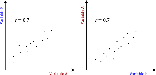
The Pearson product-moment correlation does not take into consideration whether a variable has been classified as a dependent or independent variable. It treats all variables equally. For example, you might want to find out whether basketball performance is correlated to a person's height. You might, therefore, plot a graph of performance against height and calculate the Pearson correlation coefficient. Lets say, for example, that r = .67. That is, as height increases so does basketball performance. This makes sense. However, if we plotted the variables the other way around and wanted to determine whether a person's height was determined by their basketball performance (which makes no sense), we would still get r = .67. This is because the Pearson correlation coefficient makes no account of any theory behind why you chose the two variables to compare. This is illustrated below:
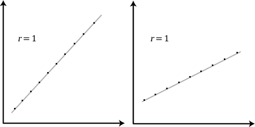
Does the Pearson correlation coefficient indicate the slope of the line?
It is important to realize that the Pearson correlation coefficient, r, does not represent the slope of the line of best fit. Therefore, if you get a Pearson correlation coefficient of +1 this does not mean that for every unit increase in one variable there is a unit increase in another. It simply means that there is no variation between the data points and the line of best fit. This is illustrated below:

What assumptions does Pearson's correlation make?
There are five assumptions that are made with respect to Pearson's correlation:
- The variables must be either interval or ratio measurements (see our Types of Variable guide for further details).
- The variables must be approximately normally distributed (see our Testing for Normality guide for further details).
- There is a linear relationship between the two variables (but see note at bottom of page). We discuss this later in this guide (jump to this section here).
- Outliers are either kept to a minimum or are removed entirely. We also discuss this later in this guide (jump to this section here).
- There is homoscedasticity of the data. This is discussed later in this guide (jump to this section here).
How can you detect a linear relationship?
To test to see whether your two variables form a linear relationship you simply need to plot them on a graph (a scatterplot, for example) and visually inspect the graph's shape. In the diagram below, you will find a few different examples of a linear relationship and some non-linear relationships. It is not appropriate to analyse a non-linear relationship using a Pearson product-moment correlation.
Comparison with regression
Comparison with regression
Correlation is almost always used when you measure both variables. It rarely is appropriate when one variable is something you experimentally manipulate.
Linear regression is usually used when X is a variable you manipulate (time, concentration, etc.)