SPSS NON-parametric statistics

SPSS has some useful syntax as well as menu to compute non-parametric statistics.

Chi-square: he Chi-Square Test procedure is useful in cross tabulated data.

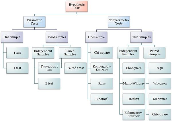
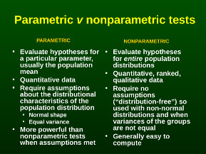
Nonparametric methods do not require distributional assumptions such as normality. They often are based on ranks. SPSS provides the list of nonparametric methods as shown on the left, which are Chi-square, Binomial, Runs, 1-Sample Kolmogorov-Smirnov, Independent Samples and Related Samples.

My Key-note address for Seminar on 'Research and Application of Checklist'

Good Morning

1.   Mr. Soumen Chatterji, Director, IIP, Kolkata, Mr. Amarnath Chatterji, chief manager, IIP, Kolkata, Dr. Rama Mallik, Head Department of Psychological Testing and Counselling, Prof. Anjali Ray, Ex-Professor, Department of Applied Psychology, CU and convener, Indian School Psychology Association,West Bengal, Dr. Rajarshi Neogi, Associate Professor, Dept. of Psychiatry, R.G.Kar Medical College and Hospital,  and distinguished guests and delegates of this one day seminar on 'Research and Application of checklist' . I deeply acknowledge the trust bestowed on me . Besides I acknowledge your immense and continuing contribution in spreading different measurement principles of Psychology through workshops, seminars and journals. I have long association with your institute since the era of Professor S. Chatterjee (the founder of the Institute) and Professor Manjula Mukerjee. I am privileged getting their continuous support on my research activities in the Indian Statistical Institute. 

2. I belong to the Psychology Research Unit of the Indian Statistical Institute, the institute of National Importance. The Unit is engaged in development of different psychometric tools for collection and assessment of complex multi-dimensional psychological data and in development of theory. Checklist is one of the psychometric tools. 


3. I have divided my key note speech into three sections – myth about checklist, my research on application of checklist and my activities as state secretary of InSPA. My intention is to minimize the errors and maximizing strength of checklist.

4. One major myth is checklist is hypothesis testing data coolection tool so checklist can not be costructed after data collection. I personally collected large number of drawing from the tribal children living in the forests of Tripura. In my picture drawing test, I constructed checklist and tested its inter rater reliability. In another research  on archive data of psychiatric disorders, I have shown how checklist can be used in data mining when data are random and non-hypothetical. Second myth is checklist is only for data collection. This is not true as Checklist is important for risk management. It prevents the user from major danger. For example, in surgery, checklist is used to improve safety surgery and to reduce death and complications for the surgery. World health Organization has introduced surgical safety checklist in November,2010.  The third myth is checklist is unnecessary as human memory is sufficient. Keep in mind that human memory has 
some potential limitations. And in danger, human memory is seriously distracted. Therefore, checklist acts as aid to reduce memory pressure and it prevents from memory distraction. Finally, it organizes our cognitive factors to achieve the goal systematically and safely. Checklist  helps to ensure consistency and completeness in carrying out a task. There are large number of psychiatric disorders in which clinical observation is recorded in the checklist. Later on degree of severity and prognosis are estimated by matching with the norm. One example is Mini Mental Status Examination test or (MMSE). Checklist is useful instrument for diagnosis of some pervasive developmental disorders like autism.  Before construction of any psychological test or questionnaire, domain wise behavior sampling is important in order to design the instrument. Checklist can be used to explore the items. In behavioural training, trainers use checklist.  Researchers involved  in action research can use checklist in school psychology.

5.  I used checklist for research purposes in 1998 in order to develop computer algorithms for construction of aptitude test battery. I published few researches in the journal. Some are - Ranking General aptitudes for success in computer programming,  Aptitude Importance Profile Similarity of Computer Programmers Across Different Organizations, Computer programming job analysis, What do computer programmers want for job satisfaction. Dr.Rama Manna was co-author of my first paper. In this study, I collected data through checklist. Later I developed checklist after data collection. First one is for Development of picture drawing test to assess consciousness layers of tribal children of Tripura. And the second one is to map association of Psychiatric complaints and the diagnostic classification. Today, in my presentation, I will show my researches.

It is nice to note that Indian School Psychology Association has been kindly agreed to be associated with this seminar. As Secretary for the State convener of InSPA, I am requesting you to be the member of InSPA. Here the word school covers any academic institution not the institution for children only.

6.  West Bengal chapter of InSPA is very dynamic and actively engaged in knowledge dissemination being associated with Workshop, Conference etc. The central body of InSPA under the leadership of Professor Panch Ramalingam regularly conducted conferences at the National and International levels. 7^th International Conference will be held in November at Mysore in this year.

7. I strongly believe that all the speakers will enlighten you different thoughts about research and application of checklist from different perspectives.

Thank you.  

http://isacabangalore.org/isacabc/main/media/downloads/2011conf/10inauguralspeech.pdf

Discriminant function analysis (P-2)

5. Basic assumptions
5.2. Prediction
5.2.1. Least square and Residuals
5.2.2 Simple and Multiple Regression
5.3 Theory of Variates
5.2.1 B coefficients
5.2.2 Beta coefficients
5.4 Discriminant function
5.4.1 Centroid
5.4.2 Wilks’ Lambda
5.4.3. Canonical Correlation


5.2 Prediction:      A statement about what you think will or might happen in the future. A prediction is what someone thinks will happen. A prediction is a forecast, but not only about the weather. Pre means “before” and “diction” has to do with talking. So a prediction is a statement about the future. It's a guess, sometimes based on facts or evidence, but not always.

5.2.1.  Least square and Residuals:

The most important application is in data fitting. The best fit in the least-squaressense minimizes the sum of squared residuals. A residual is the difference between an observed value, and the fitted value provided by a model. The method of least squares can also be derived as a method of moments estimator.

5.2.2 Simple and Multiple regression

Regression generates what is called the "least-squares" regression line. The regression line takes the form:  = a + b*X, where a and b are both constants,  (pronounced y-hat) is the predicted value of Y and X is a specific value of the independent variable. Such a formula could be used to generate values of  for a given value of X. For example, suppose a = 10 and b = 7. If X is 10, then the formula produces a predicted value for Y of 45 (from 10 + 5*7). It turns out that with any two variables X and Y, there is one equation that produces the "best fit" linking X to Y. In other words, there exists one formula that will produce the best, or most accurate predictions for Y given X. Any other equation would not fit as well and would predict Y with more error. That equation is called the least squares regression equation.

But how do we measure best? The criterion is called the least squares criterion and it looks like this:

You can imagine a formula that produces predictions for Y from each value of X in the data. Those predictions will usually differ from the actual value of Y that is being predicted (unless the Y values lie exactly on a straight line). If you square the difference and add up these squared differences across all the predictions, you get a number called the residual or error sum or squares (or SS_error). The formula above is simply the mathematical representation of SS_error. Regression generates a formula such that SS_error is as small as it can possibly be. Minimising this number (by using calculus) minimises the average error in prediction.

Y=a+bX-e

Multiple regression is an extension of simple linearregression. It is used when we want to predict the value of a variable based on the value of two or more other variables. The variable we want to predict is called the dependent variable (or sometimes, the outcome, target or criterion variable).

Multiple regression analysis is a powerful technique used for predicting the unknown value of a variable from the known value of two or more variables- also called the predictors.

Confidence interval

http://faculty.cas.usf.edu/mbrannick/regression/Prediction.html

5.3 Theory of variates

a quantity having a numerical value for each member of a group, especially one whose values occur according to a frequency distribution.It is the weight to each array variable.

5.3.1 b-coefficient

Beta coefficient :

In statistics, standardized coefficients or beta coefficients are the estimates resulting from a regression analysis that have been standardized so that the variances of dependent and independent variables are same.

Standardized coefficients refer to how many standard deviations a dependent variable will change, per standard deviation increase in the predictor variable.
     For univariate regression, the absolute value of the standardized coefficient equals the correlation coefficient.
    Standardization of the coefficient is usually done to answer the question of which of the independent variables have a greater effect on the dependent variable in a multiple regression analysis, when the variables are measured in different units of measurement (for example, income measured in dollars and family size measured in number of individuals).

5.4 Discriminant function

Discriminant function:
A function of several variates used to assign items into one of two or more groups.
    The function for a particular set of items is obtained from measurements of the variates of items which belong to a known group.

A particular combination of continuous variable test results designed to achieve separation of groups; for example, a single number representing a combination of weighted laboratory test results designed to discriminate between clinical classes.

Example
Any algorithm or assessment tool to evaluate disease severity or guide clinical or administrative decisions in health care. In gastroenterology, e.g., a discriminant function is commonly used to gauge the severity of alcoholic hepatitis. It uses two variables, the patient's measured protime (PT) and total serum bilirubin level. The difference between the patient's PT and the control PT is multiplied by 4.6 and added to the bilirubin level. If the derived number is greater than 32, the patient may benefit from treatment with corticosteroids or pentoxifylline.

5.4.1. Centroid

The method of discriminant function analysis (DFA) introduces a new concept-- i.e., the centroid.  A centroid is a value computed by finding the weighted average of intercepts for a set of regression equations.  A centroid is mapped in 3 dimensional space.

In DFA as in principal components analysis and factor analysis, a constructed variance pool is created from the calculation of all possible pair wise regression coefficients, using all predictor variables.  Each equation includes a y intercept, respectively.  The weighted averaging of predicted Y values results in C, the centroid. 

All possible pair wise calculations of correlations among predictors are completed.  Standardized regression coefficients are next computed.  The best weighted combination of predictors is identified and the first function is repeated.

The process of extracting weighted combinations of predictors continues until all variance shared by predictors has been extracted.

Each weighted combination of predictors describes a linear equation that defines a discrminant function.

A centroid for each function is computed at each step of the calculation.

For example, C first = a + bx1,x2 + a + bx,x + a + bx,x

Centroid 2 through Centroid 5 would be computed in the same way.  C 6 would be an error function expressing residual variation.

Functions are also computed, each as a vector or set of loadings that discrminate the three learning styles.  If a set of functions were computed that discrminated the 3 styles, it might look like this.

5.4.2 Willa's. Lambda

In statistics, Wilks's lambda distribution(named for Samuel S. Wilks), is a probability distribution used in multivariate hypothesis testing, especially with regard to the likelihood-ratio test and multivariate analysis of variance (MANOVA).
In discriminant analysis, Wilk’s lambda tests how well each level of independent variable contributes to the model. The scale ranges from 0 to 1, where 0 means total discrimination, and 1 means no discrimination. Each independent variable is tested by putting it into the model and then taking it out — generating a Λ statistic. The significance of the change in Λ is measured with an F-test; if the F-value is greater than the critical value, the variable is kept in the model.

5.4.3. Canonical correlation
   

Discriminant Function Analysis (P-1)

Contents:

Data Quality
4.1 Normality
4.2 Outlier
4.3 Correlation
4.4 Regression
5. Basic assumptions
5.1. Classification theory (false positive and negative)
5.1.1. Variance, ANOVA

5.1.2 MANOVA

What is Discriminant function analysis ?
A statistical discrimination of classification problem consists in assigning or classifying an individual or group of individuals to one of several known or unknown alternative populations on the basis of several measurements on the individual and samples from the unknown populations. For example, a linear combination of the measurements, called the linear discriminator or discriminant function, is constructed on the basis of its value the individual is assigned to one or the other of two populations. 

Discriminant function analysis is a statistical analysis to predict a categorical dependent variable (called a grouping variable) by one or more continuous or binary independent variables (called predictor variables).The main purpose of a discriminant function analysis is to predict group membership based on a linear combination of the interval variables. The procedure begins with a set of observations where both group membership and the values of the interval variables are known. DFA is different from MDA. MDA is a statistical technique used to reduce the differences between variables in order to classify them into a set number of broad groups. Discriminant function analysis is reversed of multivariate analysis of variance (MANOVA). In MANOVA, the independent variables are the groups and the dependent variables are the predictors.

Assumptions

Dependent and Independent Variables

• The dependent variable should be categorized by m (at least 2) text values (e.g.: 1-good student, 2-bad student; or 1-prominent student, 2-average, 3-bad student). If the dependent variable is not categorized, but its scale of measurement is interval or ratio scale, then we should categorize it first. For instance the average scholastic record is measured by ratio scale, however, if we categorize them as students with average scholastic record over 4.1 are considered good, between 2.5 and 4.0 they are average, and below 2.5 the students are bad, this variable will fulfill the requirements of discriminant analysis.
• However, we can ask: why did students over 4.1 are known as good student? Why 2.5 is the bound to consider the students bad? Due to this subjective categorization the analysis can be biased, or the correlation coefficients can be under- or overestimated. To remedy this, try to create similar size of categories. It is easier by creating graph about the distribution of dependent variables or relying on prior information. Statistical software, which contains discriminant analysis, such as SPSS, has an option, which recodes variables. However, it is more significant using already categorical variables, because in other case, we will lose some information. In case of non-categorical variables it would be better to use regression analysis instead of discriminant analysis.
• Independent variables should be metric. We do not have to standardize variables for discriminant analysis, because the unit of measures does not have decisive influence. Therefore, any metric variable can be selected for independent variable. If we have a sufficient number of quantitative variables, we can build dichotomies or ordinal scaled variables with at least 5 categories in the model (Sajtos – Mitev, 2007).

Normality

http://www.muelaner.com/wp-content/uploads/2013/07/Standard_deviation_diagram.png

• ·         The mean, median, and mode of a normal distribution are equal. The area under the normal curve is equal to 1.0. Normal distributions are denser in the center and less dense in the tails. Normal distributions are defined by two parameters, the mean (μ) and the standard deviation (σ).
• ·         The Standard Normal curve, shown here, has mean 0 and standard deviation 1. If a dataset follows a normal distribution, then about 68% of the observations will fall within of the mean , which in this case is with the interval (-1,1).
• ·         As far as I understand, attention should be paid to the normal distribution of variables along with the size.

    OUTLIER

•  It refers to a person or thing situated away or detached from the main body or system.In statistics, an outlier is an observation point that is distant from other observations. 
• An outlier may be due to 
• variability in the measurement or 
• it may indicate experimental error; the latter are sometimes excluded from the data set.
• sampling error

MEASUREMENT ERRORS

• Measurement errors can be divided into two components: random error and systematic error
• Random errors are errors in measurement that lead to measurable values being inconsistent when repeated measurements of a constant attribute or quantity are taken. 
• Systematic errors are errors that are not determined by chance but are introduced by an inaccuracy (involving either the observation or measurement process) inherent to the system.
• Systematic error may also refer to an error with a nonzero mean, the effect of which is not reduced when observations are averaged.
• Sources of systematic error may be 
• imperfect calibration of measurement instruments (zero error)
• changes in the environment which interfere with the measurement process 
•  imperfect methods of observation 
• Random errors may ocuur from non-sampling errors ( the errors are not due to sampling)
• Non-sampling errors in survey estimates can arise from:
• Coverage errors, such as failure to accurately represent all population units in the sample, or the inability to obtain information about all sample cases;
• Response errors by respondents due for example to definitional differences, misunderstandings, or deliberate misreporting;
• Mistakes in recording the data or coding it to standard classifications;
• Other errors of collection, nonresponse, processing, or imputation of values for missing or inconsistent data.

Measurement error can cause statistical error.Statistical error is the amount by which an observation differs from its expected value, the latter being based on the whole population from which the statistical unit was chosen randomly. For example, if the mean height in a population of 21-year-old men is 1.75 meters, and one randomly chosen man is 1.80 meters tall, then the "error" is 0.05 meters; if the randomly chosen man is 1.70 meters tall, then the "error" is −0.05 meters. The expected value, being the mean of the entire population, is typically unobservable, and hence the statistical error cannot be observed either.

Sample size: it is a general rule, that the larger is the sample size, the more significant is the model. The ratio of number of data to the number of variables is also important. The results can be more generalized if we have larger number of data for one variable. As a “rule of thumb”, the maximum number of independent variables is n - 2, where n is the sample size. Moreover, the smallest sample size should be at least 20 for a few (4 or 5) predictors (Poulsen – French, 2003). It is best to have 4 or 5 times, or according to some experts (Sajtos – Mitev, 2007) 10 times as many observations than independent variables. Multivariate normal distribution: it is the most frequently used distribution in statistics. In case of normal distribution, the estimation of parameters is easier, because the parameters can be defined according to the density or distribution function. It can be tested by histograms of frequency distributions or hypothesis testing. Note that violations of the normality assumption are usually not "fatal," as long as non-normality n is caused by skewness and not outliers (Tabachnick – Fidell, 1996). Non-normality can be caused by wrong scales, too (Sajtos – Mitev, 2007). As a sample size increases, the shape of the sampling distribution becomes normal. Outliers: discriminant analysis is highly sensitive for outliers, because the extreme values have a great influence on the mean, standard deviation and the statistical significance as well. In a one-variable case outliers can be defined by quartiles or boxplot, however in a multivariate case it is better to use Mahalanobis distance. Using Mahalanobis distance we can measure the distance between the cases and the centroid for each group, which difference is based on the correlation between variables. Every case will belong to a group for which its Mahalanobis distance is smallest (Hajdu, 2003). The outermost cases are regarded as outliers. For reasonable results we have to handle the problem of outliers, mainly it is better to eliminate them. Homoskedasticity: the constant variance and homogenous covariance matrices across groups are the assumptions for discriminant analysis as well. Heteroscedasticity can be caused by outliers. It can be evaluated through scatterplots of variables or the frequently used Box’s M test, which is a hypothesis testing for discriminant analysis. Box's M uses the F distribution. If p<0.05, then the variances are significantly different, thus the probability value of this F should be greater than 0.05 to demonstrate that the assumption of homoscedasticity is upheld. The test is sensitive for multivariate normal distribution. In other case using Box’s M measure is not reasonable. However, discriminant analysis can be robust even when the homoscedasticity is violated. Where sample size is large, even small differences in covariance matrices may be found significant by Box's M, when in fact no substantial problem of violation of assumptions exists. Therefore, we should also look at the log determinants of the group covariance matrices, which are printed along with Box's M. If the group log determinants are similar, then a significant Box's M for a large sample is usually ignored. Dissimilar log determinants indicates violation of the assumption of equal variance covariance matrices, leading to greater classification errors (specifically, discriminant analysis will tend to classify cases in the group with the larger variability). When violation occurs, quadratic discriminant analysis may be used (see also: http://faculty.chass.ncsu.edu/garson/PA765/discrim.htm). Multicollinearity: independent variables should be correlated to the dependent variable, however there must be no correlation between the independent variables, because it can bias the results of analysis. In case of strong multicollinearity we cannot discriminate, because the highly correlated variables would have higher role than the others. To eliminate the bias-effect we need to exclude the disturbing variables from the analysis, or create a principle component of the correlated variables. Using Mahalanobis distance we prove the independence of variables. Linearity: we assume a linear relation between the independent variables, which can be tested by scatterplot. This assumption does not take into account unless transformed variables are added as additional independent variables. Other assumptions are (Sajtos – Mitev, 2007): Independence: not only the explanatory variables, but also all cases must be independent. Therefore, panel, longitudinal research, or pre-test data cannot be used for discriminant analysis. Mutually exclusive groups: all cases must belong to one group and every case of the dependent variable must belong to only one group. Group size: the size of groups should be pretty much the same and every group should contain at least 2 cases. If this assumption is violated, it will be better to use logistic regression instead of discriminant analysis. However, statistical programs, such as SPSS help to get significant results as well if the group sizes are not equal. The correction based on the group size can be optionally selected, thus we eliminate the problems caused by non-equal groups.

 Prev

 The assumptions of discriminant analysis are the same as those for MANOVA. The analysis is quite sensitive to outliers and the size of the smallest group must be larger than the number of predictor variables. Multivariate normality: Independent variables are normal for each level of the grouping variable.

Normality:

Correlation

a ratio between +1 and −1 calculated so as to represent the linear interdependence of two variables or sets of data.

Pearson Product-Moment Correlation

What does this test do?

The Pearson product-moment correlation coefficient (or Pearson correlation coefficient, for short) is a measure of the strength of a linear association between two variables and is denoted by r. Basically, a Pearson product-moment correlation attempts to draw a line of best fit through the data of two variables, and the Pearson correlation coefficient, r, indicates how far away all these data points are to this line of best fit (i.e., how well the data points fit this new model/line of best fit).

What values can the Pearson correlation coefficient take?

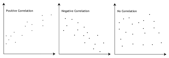
The Pearson correlation coefficient, r, can take a range of values from +1 to -1. A value of 0 indicates that there is no association between the two variables. A value greater than 0 indicates a positive association; that is, as the value of one variable increases, so does the value of the other variable. A value less than 0 indicates a negative association; that is, as the value of one variable increases, the value of the other variable decreases. This is shown in the diagram below:

How can we determine the strength of association based on the Pearson correlation coefficient?

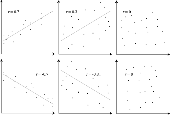
The stronger the association of the two variables, the closer the Pearson correlation coefficient, r, will be to either +1 or -1 depending on whether the relationship is positive or negative, respectively. Achieving a value of +1 or -1 means that all your data points are included on the line of best fit – there are no data points that show any variation away from this line. Values for r between +1 and -1 (for example, r = 0.8 or -0.4) indicate that there is variation around the line of best fit. The closer the value of r to 0 the greater the variation around the line of best fit. Different relationships and their correlation coefficients are shown in the diagram below:

Join the 10,000s of students, academics and professionals who rely on Laerd Statistics.TAKE THE TOUR PLANS & PRICING

Are there guidelines to interpreting Pearson's correlation coefficient?

Yes, the following guidelines have been proposed:

	Coefficient, r
Strength of Association	Positive	Negative
Small	.1 to .3	-0.1 to -0.3
Medium	.3 to .5	-0.3 to -0.5
Large	.5 to 1.0	-0.5 to -1.0

Remember that these values are guidelines and whether an association is strong or not will also depend on what you are measuring.

Can you use any type of variable for Pearson's correlation coefficient?

No, the two variables have to be measured on either an interval or ratio scale. However, both variables do not need to be measured on the same scale (e.g., one variable can be ratio and one can be interval). Further information about types of variable can be found in our Types of Variable guide. If you have ordinal data, you will want to use Spearman's rank-order correlation or a Kendall's Tau Correlation instead of the Pearson product-moment correlation.

Do the two variables have to be measured in the same units?

No, the two variables can be measured in entirely different units. For example, you could correlate a person's age with their blood sugar levels. Here, the units are completely different; age is measured in years and blood sugar level measured in mmol/L (a measure of concentration). Indeed, the calculations for Pearson's correlation coefficient were designed such that the units of measurement do not affect the calculation. This allows the correlation coefficient to be comparable and not influenced by the units of the variables used.

What about dependent and independent variables?

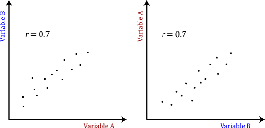
The Pearson product-moment correlation does not take into consideration whether a variable has been classified as a dependent or independent variable. It treats all variables equally. For example, you might want to find out whether basketball performance is correlated to a person's height. You might, therefore, plot a graph of performance against height and calculate the Pearson correlation coefficient. Lets say, for example, that r = .67. That is, as height increases so does basketball performance. This makes sense. However, if we plotted the variables the other way around and wanted to determine whether a person's height was determined by their basketball performance (which makes no sense), we would still get r = .67. This is because the Pearson correlation coefficient makes no account of any theory behind why you chose the two variables to compare. This is illustrated below:

Does the Pearson correlation coefficient indicate the slope of the line?

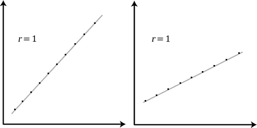
It is important to realize that the Pearson correlation coefficient, r, does not represent the slope of the line of best fit. Therefore, if you get a Pearson correlation coefficient of +1 this does not mean that for every unit increase in one variable there is a unit increase in another. It simply means that there is no variation between the data points and the line of best fit. This is illustrated below:

TAKE THE TOUR

PLANS & PRICING

What assumptions does Pearson's correlation make?

There are five assumptions that are made with respect to Pearson's correlation:

1. The variables must be either interval or ratio measurements (see our Types of Variable guide for further details).
2. The variables must be approximately normally distributed (see our Testing for Normality guide for further details).
3. There is a linear relationship between the two variables (but see note at bottom of page). We discuss this later in this guide (jump to this section here).
4. Outliers are either kept to a minimum or are removed entirely. We also discuss this later in this guide (jump to this section here).
5. There is homoscedasticity of the data. This is discussed later in this guide (jump to this section here).

How can you detect a linear relationship?

To test to see whether your two variables form a linear relationship you simply need to plot them on a graph (a scatterplot, for example) and visually inspect the graph's shape. In the diagram below, you will find a few different examples of a linear relationship and some non-linear relationships. It is not appropriate to analyse a non-linear relationship using a Pearson product-moment correlation.

Comparison with regression

Correlation is almost always used when you measure both variables. It rarely is appropriate when one variable is something you experimentally manipulate.

Linear regression is usually used when X is a variable you manipulate (time, concentration, etc.)

My Father

My father was freedom fighter. He fought against British. He later on came to West Bengal after partition 

with his parents, two brothers and sisters from Mymensingha, the place of arts and literature.  His village 

name was Gachihata. 











 








There were three times of Bengal partitions. First was in 1905 by Lord Curzon and in 1947 following Radcliffe line. Third was in 1971 during the period of Sheikh Mujibur Rahman and Indira Gandhi.
Possibly he came to West Bengal in 1947. Like other migrants he was penniless. He had lost own properties in then East Bengal like others. He studied Commerce staying in a mess. Though he liked History very much as I observed from his collections. Poverty attacked him like other migrants. He managed education through paper distribution and writing on some daily newspaper using pseudoname as freelance writer.
My father was good orator and teacher. He was influenced by then communism. Later he was principal of one commercial college close to Sealdaha Rail station. It seems to be George Telegraph. He was good student in commerce. He was typist and shorthand specialist.
He knew the Educational pain in poverty. He always thought of others. He wanted dissemination of his knowledge for career development of others. So he started one Institute for typing and shorthand nearby Prachi cinema hall in Kolkata. I was fortunate in learning typing and shorthand at this Institute but he could not see as he passed away when I was one or two months old.
His marriage was just like story. My mother was metron of B. R. Singh hospital. She rescued my father from Morgue. She was Christian. My Grandfather was conservative Hindu but he gladly accepted my mother. To me, my mother was saviour. She nursed my father like other patients. She was dominant and confident in her nursing. So when he didn't find my father on bed and knew that the dead body was shifted to the morgue, she could not believe. Finally he brought declared dead body and gave life. My Grandfather addressed my mother 'Sabitri' following the mythology of Sabitri and Satyaban.
My Grandfather Late Nishi Bhushan Dutta Roy was writer but he wrote about religious issues. He wrote one book ' 'Mayur Mukut Lila Mrito'. He roamed around Himalayas met many sages and spent life as sage. In this book he described his religious life. My Grand mother was close relative of Late Upendra Kishore Roy Choudhury, father of late Satyajit Roy.

Rabindra Sangeet in Psychological counselling

Why Rabindra Sangeet in Psychological counselling  ?
Success of Psychological Counselling depends on situational and dispositional attributions. Sometimes situational attributes become more powerful and client feels less control over it. Again when client attributes self for the illness, he or she is more stressed. Rabindra Sangeet
never attributes self or other/s for illness. Rather it creates illness reasoning and guided imageries to overcome the illness.So illness perception can be changed through the regimen coming from within.

R-Programming

Reading Table data from Desktop 

File name; Testdata
Source:C:\Users\Dr.D.D.Roy\Desktop\Testdata.txt

R command:

1. test <- read.table("C:/Users/Dr.D.D.Roy/Desktop/Testdata.txt", header=TRUE)

Path direction has been changed from | to /. Header indicates name of column variable.

2. list(test)

List command for display of data. The data has been stored in the array named 'test'

> list(test)

[[1]]

  Price Floor Area Rooms Age Cent.heat

1 52.00   111  830     5 6.2        no

2 54.75   128  710     5 7.5        no

3 57.50   101 1000     5 4.2        no

4 57.50   131  690     6 8.8        no

5 59.75    93  900     5 1.9       yes

Reading no of rows and columns


> dim(test)
[1] 5 6
> str(test)
'data.frame':   5 obs. of  6 variables:
 $ Price    : num  52 54.8 57.5 57.5 59.8
 $ Floor    : num  111 128 101 131 93
 $ Area     : int  830 710 1000 690 900
 $ Rooms    : int  5 5 5 6 5
 $ Age      : num  6.2 7.5 4.2 8.8 1.9
 $ Cent.heat: Factor w/ 2 levels "no","yes": 1 1 1 1 2

Help command

Before we get deeper into the use of R, it is good to know how to seek help when we get stuck. Two functions are illustrated here. If you know the name of a function or the topic, you may use the function help(…) with your function name or topic inside the parenthesis. For example, if you are interested in the function plot(), you can type

> help(plot)

and it will pop-up a help manual for plot function. This can be done more quickly by typing a question mark in front of the function in question.

> ?plot

Sometimes, you may want to find something related to a certain keyword. Then you may find help.search() useful. Function help.search() will search for all the functions that have the word you specified in their help document such as name, title, concept, keyword. For example,

> help.search("sort")

will list all functions that have the word 'sort' as an alias or in their title. The dunction help.search() also has a shortcut consisting of two question marks preceding the keyword (e.g., ??sort). If you want to learn more about the help function, you may type help(help). Besides the official help pages, you can also explore the Internet, which has many resources.

More commands

http://www.personality-project.org/r/r.commands.html

Q1. What is R?

Why Use R?

If you currently use another statistical package, why learn R?

It's free! If you are a teacher or a student, the benefits are obvious.

It runs on a variety of platforms including Windows, Unix and MacOS.

It provides an unparalleled platform for programming new statistical methods in an easy and straightforward manner.

It contains advanced statistical routines not yet available in other packages.

It has state-of-the-art graphics capabilities.

Obtaining R

R is available for Linux, MacOS X, and Windows (95 or later) platforms. Software can be downloaded from one of the Comprehensive R Archive Network(CRAN) mirror sites.

Feedback

I constantly strive to improve these pages. Feedback and suggestions are always welcome! 

- Rob Kabacoff