Wednesday, December 5, 2018

Rank data analysis Hazaribagh


Powerpoint presentation of R script

https://www.slideshare.net/ddroy/revisiting-the-fundamental-concepts-and-assumptions-of-statistics-pps

R is a free and powerful programming language and environment for statistical computing, data exploration, data analysis and data visualization that is supported by the R Foundation for Statistical Computing. R was created by Ross Ihaka and Robert Gentleman at the University of Auckland, New Zealand. Graphics of R is useful for Data visualization. For data examination, data visualization locates the errors in data structure with respect to outliers, relations among different data sets. R allows extremely flexible use of data structure. Furthermore, R includes user friendly logical functions. R can deal with problems in a wide range of field as it has more than 75000 packages. For example,psych package is useful for examining psychometric properties of psychological instruments. The package can be downloaded from internet for temporary periods.

Download

The website is :
Cran Mirror​: https://cran.r-project.org/bin/windows/base/
R-Studio​: https://www.rstudio.com/products/rstudio/download/
Download of R is followed by the download of cran mirror.


Data analysis command (uni and bivariate)


  1. value=read.csv(choose.files(),header=T,sep=",")
  2. x=read.table(file="clipboard",header=T,sep="\t")
  3. write.table(x,file="copydata",sep="\t")
  4. write.csv(pathvalue)# writing data on the screen
  5. write.csv(pathvalue[1])# data examination
  6. write.csv(pathvalue,file="pathvalue.csv")# writing on the drive
  7. c=read.csv(file="clipboard",header=T,sep="\t")
  8. scan()
  9. readline()
  10. View(x)
  11. xx=na.omit(x)
  12. NROW(value)
  13. length(value)
  14. str(value)
  15. names(value)
  16. value[2] # name of the trainees
  17. summary(value)
  18. median(value$Age,na.rm=T)
  19. range(value$Age,na.rm=T)
  20. mean(value$Age,na.rm=T)
  21. tx=table(value$Age)
  22. xec=cut(as.numeric(value$EMOTIONAL.CONTROL),breaks = 2, labels=c("HighEC", "LOWEC"))
  23. table(xec) # highec and lowec
  24. table(value[4]) #frequency of male and female
  25. pie(table(value[4])) # multiple functions in single command
  26. boxplot(value$Age~value$Sex)
  27. xec=cut(as.numeric(value$EMOTIONAL.CONTROL),breaks = c(0,5,10,14),labels=c("high", “moderate”,”less”))
  28. wilcox.test(value$Age~agecateg)
  29. kruskal.test(value$Age~agecateg)
  30. pathvalue=data.frame(value[12:26]) # data frame of pathoriented values
  31. pathvalue[1:5,] # first 5 data of pathoriented values
  32. file.info(dir())#check the file
  33. pathvalue$EMOTIONAL.CONTROL==03# error identified
  34. cor(x,use="all.obs",method="spearman")
  35. cor(x,use="all.obs",method="kendall")
  36. Which(is.na(pathvalue[2]))
  37. sexcode=replace(x$SEX.CODE,x$SEX.CODE == "1", "male")
  38. agecode=factor(x$AGE.CODE, levels=c(1,2), labels=c("13-30","31-48>"))
  39. x=subset(patients,patients$Classification==4)

Matrix

Generally we are dealing with single dimensional data. When single dimensional data are converted into two,three or more dimensions, it becomes matrix.

xx=matrix(x$age, nrow =198,ncol =2)

Here, x$age is single dimensional data.  It becomes 2 dimensions.

Loop

for(i in 1:45) {
   
    t=(table(climate[i]))
    print(i)
    print(t)
   
}


9. data.frame(value$Name,value$Age<35,value$Age)

Tuesday, October 23, 2018

Research method in hearing impairment

Research settings are important to minimize effects of intervening variables on the dependent variable/s. Broadly there are 3 settings - controlled condition, field settings and natural settings. 

circulatory disturbance to the cochlea, viral infection, and autoimmune disease, exposure to intense sounds has been shown to cause permanent damage to the auditory system; 

https://www.jove.com/video/53264/neuro-rehabilitation-approach-for-sudden-sensorineural-hearing-loss

Experimental design 

https://www.okstate.edu/ag/agedcm4h/academic/aged5980a/5980/newpage2.htm


Line chart

Age wise change


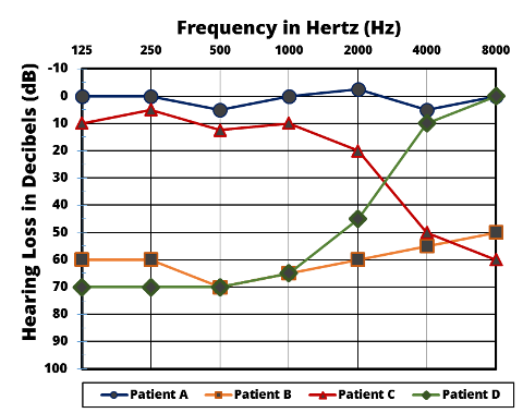
Figure 1. Illustrating presbycusis - age related hearing loss. M : men, W : women
 (after Prof L Beranek)

Ref: http://www.pykett.org.uk/arhlandob.htm


Patient wise comparison


Sensitivity and Specificity


  • Sensitivity (also called the true positive rate, the recall, or probability of detection[1] in some fields) measures the proportion of actual positives that are correctly identified as such (e.g., the percentage of sick people who are correctly identified as having the condition).
  • Specificity (also called the true negative rate) measures the proportion of actual negatives that are correctly identified as such (e.g., the percentage of healthy people who are correctly identified as not having the condition).

Sensitivity therefore quantifies the avoiding of false negatives, and specificity does the same for false positives

a false positive is an error in data reporting in which a test result improperly indicates presence of a condition, such as a disease (the result is positive), when in reality it is not present, while a false negative is an error in which a test result improperly indicates no presence of a condition (the result is negative), when in reality it is present.


Hearing screening instrument
https://consultgeri.org/try-this/general-assessment/issue-12.pdf

Sensitivity was measured in the group of participants identified as having bilateral hearing loss on audiometry, defined as the proportion who reported hearing loss. Specificity was measured in the group of participants identified as having normal hearing in both ears, defined as the proportion who reported normal hearing. Positive predictive value (PPV) is the probability that the question would correctly identify a person as having bilateral hearing impairment. Negative predictive value (NPV) indicates the probability that the question would correctly identify a person whose hearing was normal. Differences between measured and estimated prevalence rates (using the referent standard and self-report data, respectively), were tested for statistical significance using the McNemar statistic. 


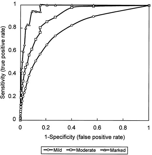
Receiver operating characteristic (ROC) curves were generated for the three severity levels of hearing loss by computing the true positive rate (sensitivity) and false positive rate (1-specificity) of the test at several cut-points, using an HHIE-S score >8. These pairs (sensitivity, 1-specificity) were then plotted to graph the ROC. The area under the ROC curve (AUC) represents the discrimination power of an HHIE-S score >8 at each level of hearing loss and varies from 0.5 (accuracy occurring by chance) to 1.0 (perfect accuracy). As the ROC curve shifts towards the left and top boundaries of the graph, the AUC is closer to 1.0.

======================================

Normal Probability Curve
Distribution of hearing loss characteristics in a clinical population. ... One-third of all records indicated normal hearing in at least one ear and one fourth had normal hearing in both ears. Mild and moderate hearing losses were equally prevalent, each contributing 40% to 45% of the cases with hearing loss.

Again, measurement involves assigning scores to individuals so that they represent some characteristic of the individuals. But how do researchers know that the scores actually represent the characteristic, especially when it is a construct like intelligence, self-esteem, depression, or working memory capacity? The answer is that they conduct research using the measure to confirm that the scores make sense based on their understanding of the construct being measured. This is an extremely important point. Psychologists do not simply assume that their measures work. Instead, they collect data to demonstrate that they work. If their research does not demonstrate that a measure works, they stop using it.

As an informal example, imagine that you have been dieting for a month. Your clothes seem to be fitting more loosely, and several friends have asked if you have lost weight. If at this point your bathroom scale indicated that you had lost 10 pounds, this would make sense and you would continue to use the scale. But if it indicated that you had gained 10 pounds, you would rightly conclude that it was broken and either fix it or get rid of it. In evaluating a measurement method, psychologists consider two general dimensions: reliability and validity.

Reliability

Reliability refers to the consistency of a measure. Psychologists consider three types of consistency: over time (test-retest reliability), across items (internal consistency), and across different researchers (inter-rater reliability).

Test-Retest Reliability

When researchers measure a construct that they assume to be consistent across time, then the scores they obtain should also be consistent across time. Test-retest reliability is the extent to which this is actually the case. For example, intelligence is generally thought to be consistent across time. A person who is highly intelligent today will be highly intelligent next week. This means that any good measure of intelligence should produce roughly the same scores for this individual next week as it does today. Clearly, a measure that produces highly inconsistent scores over time cannot be a very good measure of a construct that is supposed to be consistent.

Assessing test-retest reliability requires using the measure on a group of people at one time, using it again on the same group of people at a later time, and then looking at test-retest correlation between the two sets of scores. This is typically done by graphing the data in a scatterplot and computing Pearson’s r. Figure 5.2 shows the correlation between two sets of scores of several university students on the Rosenberg Self-Esteem Scale, administered two times, a week apart. Pearson’s r for these data is +.95. In general, a test-retest correlation of +.80 or greater is considered to indicate good reliability.

Figure 5.2 Test-Retest Correlation Between Two Sets of Scores of Several College Students on the Rosenberg Self-Esteem Scale, Given Two Times a Week Apart
Again, high test-retest correlations make sense when the construct being measured is assumed to be consistent over time, which is the case for intelligence, self-esteem, and the Big Five personality dimensions. But other constructs are not assumed to be stable over time. The very nature of mood, for example, is that it changes. So a measure of mood that produced a low test-retest correlation over a period of a month would not be a cause for concern.

Internal Consistency

A second kind of reliability is internal consistency, which is the consistency of people’s responses across the items on a multiple-item measure. In general, all the items on such measures are supposed to reflect the same underlying construct, so people’s scores on those items should be correlated with each other. On the Rosenberg Self-Esteem Scale, people who agree that they are a person of worth should tend to agree that that they have a number of good qualities. If people’s responses to the different items are not correlated with each other, then it would no longer make sense to claim that they are all measuring the same underlying construct. This is as true for behavioural and physiological measures as for self-report measures. For example, people might make a series of bets in a simulated game of roulette as a measure of their level of risk seeking. This measure would be internally consistent to the extent that individual participants’ bets were consistently high or low across trials.

Like test-retest reliability, internal consistency can only be assessed by collecting and analyzing data. One approach is to look at a split-half correlation. This involves splitting the items into two sets, such as the first and second halves of the items or the even- and odd-numbered items. Then a score is computed for each set of items, and the relationship between the two sets of scores is examined. For example, Figure 5.3 shows the split-half correlation between several university students’ scores on the even-numbered items and their scores on the odd-numbered items of the Rosenberg Self-Esteem Scale. Pearson’s r for these data is +.88. A split-half correlation of +.80 or greater is generally considered good internal consistency.

Figure 5.3 Split-Half Correlation Between Several College Students’ Scores on the Even-Numbered Items and Their Scores on the Odd-Numbered Items of the Rosenberg Self-Esteem Scale
Perhaps the most common measure of internal consistency used by researchers in psychology is a statistic called Cronbach’s α (the Greek letter alpha). Conceptually, α is the mean of all possible split-half correlations for a set of items. For example, there are 252 ways to split a set of 10 items into two sets of five. Cronbach’s α would be the mean of the 252 split-half correlations. Note that this is not how α is actually computed, but it is a correct way of interpreting the meaning of this statistic. Again, a value of +.80 or greater is generally taken to indicate good internal consistency.

Interrater Reliability

Many behavioural measures involve significant judgment on the part of an observer or a rater. Inter-rater reliability is the extent to which different observers are consistent in their judgments. For example, if you were interested in measuring university students’ social skills, you could make video recordings of them as they interacted with another student whom they are meeting for the first time. Then you could have two or more observers watch the videos and rate each student’s level of social skills. To the extent that each participant does in fact have some level of social skills that can be detected by an attentive observer, different observers’ ratings should be highly correlated with each other. Inter-rater reliability would also have been measured in Bandura’s Bobo doll study. In this case, the observers’ ratings of how many acts of aggression a particular child committed while playing with the Bobo doll should have been highly positively correlated. Interrater reliability is often assessed using Cronbach’s α when the judgments are quantitative or an analogous statistic called Cohen’s κ (the Greek letter kappa) when they are categorical.

Validity

Validity is the extent to which the scores from a measure represent the variable they are intended to. But how do researchers make this judgment? We have already considered one factor that they take into account—reliability. When a measure has good test-retest reliability and internal consistency, researchers should be more confident that the scores represent what they are supposed to. There has to be more to it, however, because a measure can be extremely reliable but have no validity whatsoever. As an absurd example, imagine someone who believes that people’s index finger length reflects their self-esteem and therefore tries to measure self-esteem by holding a ruler up to people’s index fingers. Although this measure would have extremely good test-retest reliability, it would have absolutely no validity. The fact that one person’s index finger is a centimetre longer than another’s would indicate nothing about which one had higher self-esteem.

Discussions of validity usually divide it into several distinct “types.” But a good way to interpret these types is that they are other kinds of evidence—in addition to reliability—that should be taken into account when judging the validity of a measure. Here we consider three basic kinds: face validity, content validity, and criterion validity.

Face Validity

Face validity is the extent to which a measurement method appears “on its face” to measure the construct of interest. Most people would expect a self-esteem questionnaire to include items about whether they see themselves as a person of worth and whether they think they have good qualities. So a questionnaire that included these kinds of items would have good face validity. The finger-length method of measuring self-esteem, on the other hand, seems to have nothing to do with self-esteem and therefore has poor face validity. Although face validity can be assessed quantitatively—for example, by having a large sample of people rate a measure in terms of whether it appears to measure what it is intended to—it is usually assessed informally.

Face validity is at best a very weak kind of evidence that a measurement method is measuring what it is supposed to. One reason is that it is based on people’s intuitions about human behaviour, which are frequently wrong. It is also the case that many established measures in psychology work quite well despite lacking face validity. The Minnesota Multiphasic Personality Inventory-2 (MMPI-2) measures many personality characteristics and disorders by having people decide whether each of over 567 different statements applies to them—where many of the statements do not have any obvious relationship to the construct that they measure. For example, the items “I enjoy detective or mystery stories” and “The sight of blood doesn’t frighten me or make me sick” both measure the suppression of aggression. In this case, it is not the participants’ literal answers to these questions that are of interest, but rather whether the pattern of the participants’ responses to a series of questions matches those of individuals who tend to suppress their aggression.

Content Validity

Content validity is the extent to which a measure “covers” the construct of interest. For example, if a researcher conceptually defines test anxiety as involving both sympathetic nervous system activation (leading to nervous feelings) and negative thoughts, then his measure of test anxiety should include items about both nervous feelings and negative thoughts. Or consider that attitudes are usually defined as involving thoughts, feelings, and actions toward something. By this conceptual definition, a person has a positive attitude toward exercise to the extent that he or she thinks positive thoughts about exercising, feels good about exercising, and actually exercises. So to have good content validity, a measure of people’s attitudes toward exercise would have to reflect all three of these aspects. Like face validity, content validity is not usually assessed quantitatively. Instead, it is assessed by carefully checking the measurement method against the conceptual definition of the construct.

Criterion Validity

Criterion validity is the extent to which people’s scores on a measure are correlated with other variables (known as criteria) that one would expect them to be correlated with. For example, people’s scores on a new measure of test anxiety should be negatively correlated with their performance on an important school exam. If it were found that people’s scores were in fact negatively correlated with their exam performance, then this would be a piece of evidence that these scores really represent people’s test anxiety. But if it were found that people scored equally well on the exam regardless of their test anxiety scores, then this would cast doubt on the validity of the measure.

A criterion can be any variable that one has reason to think should be correlated with the construct being measured, and there will usually be many of them. For example, one would expect test anxiety scores to be negatively correlated with exam performance and course grades and positively correlated with general anxiety and with blood pressure during an exam. Or imagine that a researcher develops a new measure of physical risk taking. People’s scores on this measure should be correlated with their participation in “extreme” activities such as snowboarding and rock climbing, the number of speeding tickets they have received, and even the number of broken bones they have had over the years. When the criterion is measured at the same time as the construct, criterion validity is referred to as concurrent validity; however, when the criterion is measured at some point in the future (after the construct has been measured), it is referred to as predictive validity (because scores on the measure have “predicted” a future outcome).

Criteria can also include other measures of the same construct. For example, one would expect new measures of test anxiety or physical risk taking to be positively correlated with existing measures of the same constructs. This is known as convergent validity.

Assessing convergent validity requires collecting data using the measure. Researchers John Cacioppo and Richard Petty did this when they created their self-report Need for Cognition Scale to measure how much people value and engage in thinking (Cacioppo & Petty, 1982)[1]. In a series of studies, they showed that people’s scores were positively correlated with their scores on a standardized academic achievement test, and that their scores were negatively correlated with their scores on a measure of dogmatism (which represents a tendency toward obedience). In the years since it was created, the Need for Cognition Scale has been used in literally hundreds of studies and has been shown to be correlated with a wide variety of other variables, including the effectiveness of an advertisement, interest in politics, and juror decisions (Petty, Briñol, Loersch, & McCaslin, 2009)[2].

Discriminant Validity

Discriminant validity, on the other hand, is the extent to which scores on a measure are not correlated with measures of variables that are conceptually distinct. For example, self-esteem is a general attitude toward the self that is fairly stable over time. It is not the same as mood, which is how good or bad one happens to be feeling right now. So people’s scores on a new measure of self-esteem should not be very highly correlated with their moods. If the new measure of self-esteem were highly correlated with a measure of mood, it could be argued that the new measure is not really measuring self-esteem; it is measuring mood instead.

When they created the Need for Cognition Scale, Cacioppo and Petty also provided evidence of discriminant validity by showing that people’s scores were not correlated with certain other variables. For example, they found only a weak correlation between people’s need for cognition and a measure of their cognitive style—the extent to which they tend to think analytically by breaking ideas into smaller parts or holistically in terms of “the big picture.” They also found no correlation between people’s need for cognition and measures of their test anxiety and their tendency to respond in socially desirable ways. All these low correlations provide evidence that the measure is reflecting a conceptually distinct construct.

Key Takeaways

Psychological researchers do not simply assume that their measures work. Instead, they conduct research to show that they work. If they cannot show that they work, they stop using them.
There are two distinct criteria by which researchers evaluate their measures: reliability and validity. Reliability is consistency across time (test-retest reliability), across items (internal consistency), and across researchers (interrater reliability). Validity is the extent to which the scores actually represent the variable they are intended to.
Validity is a judgment based on various types of evidence. The relevant evidence includes the measure’s reliability, whether it covers the construct of interest, and whether the scores it produces are correlated with other variables they are expected to be correlated with and not correlated with variables that are conceptually distinct.
The reliability and validity of a measure is not established by any single study but by the pattern of results across multiple studies. The assessment of reliability and validity is an ongoing process.
Exercises

Practice: Ask several friends to complete the Rosenberg Self-Esteem Scale. Then assess its internal consistency by making a scatterplot to show the split-half correlation (even- vs. odd-numbered items). Compute Pearson’s r too if you know how.
Discussion: Think back to the last college exam you took and think of the exam as a psychological measure. What construct do you think it was intended to measure? Comment on its face and content validity. What data could you collect to assess its reliability and criterion validity?
Cacioppo, J. T., & Petty, R. E. (1982). The need for cognition. Journal of Personality and Social Psychology, 42, 116–131. ↵
Petty, R. E, Briñol, P., Loersch, C., & McCaslin, M. J. (2009). The need for cognition. In M. R. Leary & R. H. Hoyle (Eds.), Handbook of individual differences in social behaviour (pp. 318–329). New York, NY: Guilford Press. ↵
 Previous: Understanding Psychological Measurement


Monday, October 15, 2018

Job analysis

Job characteristics

It states that there are five core job characteristics (skill variety, task identity, task significance, autonomy, and feedback) which impact three critical psychological states (experienced meaningfulness, experienced responsibility for outcomes, and knowledge of the actual results), in turn influencing work outcomes (job satisfaction, absenteeism, work motivation, etc.). The five core job characteristics can be combined to form a motivating potential score (MPS) for a job, which can be used as an index of how likely a job is to affect an employee's attitudes and behaviors.
Hackman and Oldham’s job characteristics theory proposes that high motivation is related to experiencing three psychological states whilst working:
  1. Meaningfulness of work
    That labour has meaning to you, something that you can relate to, and does not occur just as a set of movements to be repeated. This is fundamental to intrinsic motivation, i.e. that work is motivating in an of itself (as opposed to motivating only as a means to an end).
  2. Responsibility
    That you have been given the opportunity to be a success or failure at your job because sufficient freedom of action has given you. This would include the ability to make changes and incorporate the learning you gain whilst doing the job.
  3. Knowledge of outcomes
    This is important for two reasons. Firstly to provide the person knowledge on how successful their work has been, which in turn enables them to learn from mistakes. The second is to connect them emotionally to the customer of their outputs, thus giving further purpose to the work (e.g. I may only work on a production line, but I know that the food rations I produce are used to help people in disaster areas, saving many lives).
In turn, each of these critical states are derived from certain characteristics of the job:
  1. Meaningfulness of work
    The work must be experienced as meaningful (his/her contribution significantly affects the overall effectiveness of the organization). This is derived from:
    • Skill variety
      Using an appropriate variety of your skills and talents: too many might be overwhelming, too few, boring.
    • Task Identity
      Being able to identify with the work at hand as more whole and complete, and hence enabling more pride to be taken in the outcome of that work (e.g. if you just add one nut to one bolt in the same spot every time a washing machine goes past it is much less motivating than being the person responsible for the drum attachment and associated work area (even as part of a group).
    • Task Significance
      Being able to identify the task as contributing to something wider, to society or a group over and beyond the self. For example, the theory suggests that I will be more motivated if I am contributing to the whole firm’s bonus this year, looking after someone or making something that will benefit someone else. Conversely I will be less motivated if I am only making a faceless owner wealthier, or am making some pointless item (e.g. corporate give-away gifts).
  2. Responsibility
    Responsibility is derived from autonomy, as in the job provides substantial freedom, independence and discretion to the individual in scheduling the work and in determining the procedures to be used in carrying it out)
  3. Knowledge of outcomes
    This comes from feedback. It implies an employee awareness of how effective he/she is converting his/her effort into performance. This can be anything from production figures through to customer satisfaction scores. The point is that the feedback offers information that once you know, you can use to do things differently if you wish. Feedback can come from other people or the job itself.
Knowing these critical job characteristics, the theory goes, it is then possible to derive the key components of the design of a job and redesign it:
  1. Varying work to enable skill variety
  2. Assigning work to groups to increase the wholeness of the product produced and give a group to enhance significance
  3. Delegate tasks to their lowest possible level to create autonomy and hence responsibility
  4. Connect people to the outcomes of their work and the customers that receive them so as to provide feedback for learning
Ref:https://www.yourcoach.be/en/employee-motivation-theories/hackman-oldham-job-characteristics-model.php


What’s more, the theory they produced was universal and could be applied to any role. They identified the following job characteristics that must be in place to achieve employee satisfaction:
  • Skills variety: do tasks vary, and are they challenging? Or are they monotonous and too easy?
  • Task identity: do tasks have a defined beginning, middle and end? Without this, it’s hard to achieve the satisfaction of an attained goal.
  • Task significance: does the employee feel that their role has meaning?
  • Task autonomy: can individuals have a say in how they carry out their work?
  • Job feedback: are employees receiving feedback on their performance?
If a job is consciously created to be varied and meaningful, with plenty of two-way communication, the employee will be more engaged with their role. According to Hackman & Oldham, they will also have an increased sense of responsibility for their work outcomes.
The model still acknowledges the role of intrinsic motivators, as proposed by Edward Deci & Richard Ryan, which said that motivation falls on a scale that ranges from ‘extrinsic’ (controlled) to ‘intrinsic’ (autonomous). However, Hackman & Oldham place more onus on HR and management to ensure that the job creation stage hits the right notes.


Process analysis

process analyst is a specialized analyst who works with businesses to break down business processes into specific steps. This helps the company understand and improve business processesProcess analysts work on projects designed to improve quality, reduce errors and design new business processes.

A Business Process Analyst (BPA) is a specialty Business Analyst Role that involves “thinking processes”. ... Business Process Analysts have knowledge ofprocess mapping and business process reengineering. They analyse businessprocesses and workflows with the objective of finding out how they can be improved or automated.


knowldge, skill, abilties
https://en.wikipedia.org/wiki/Knowledge,_Skills,_and_Abilities


Monday, September 17, 2018

APA format for writing Doc file

From R results to APA format

https://cran.r-project.org/web/packages/apaTables/vignettes/apaTables.html


  1. Make 1 inch margins on the top, bottom, and sides.
  2. The first word in every paragraph should be indented one half inch.
  3. APA recommends using Times New Roman font, size 12.
  4. Double space the entire research paper.
  5. To create the running head/page header, insert page numbers justified to the right-hand side of the paper (do not put p. or pg. in front of page numbers)
  6. Then type “TITLE OF YOUR PAPER” justified to the left using all capital letters
  7. If your title is long, this running head title should be a shortened version of the title of your entire paper.

APA Paper Components
Your essay should include these four major sections:
  1. Title Page
  2. Abstract
  3. Main Body
  4. References
Title Page
This page should contain four pieces: the title of the paper, 

a)running head, 
b)the author’s name, 
c)institutional affiliation, 
d)an author’s note. 

*Please note that only on the title page, your page header/running head should include the words “Running Head” before your title in all capitals. The rest of the pages should not include this in the page header. It should look like this on the title page:


Abstract
On the following page, begin with the Running title.
  1. On the first line of the page, center the word “Abstract” (but do not include quotation marks).
  2. On the following line, write a summary of the key points of your research. Your abstract summary is a way to introduce readers to your research topic, the questions that will be answered, the process you took, and any findings or conclusions you drew.
  3. This summary should not be indented, but should be double-spaced and less than 250 words.
  4. If applicable, help researchers find your work in databases by listing keywords from your paper after your summary. To do this, indent and type Keywords: in italics.  Then list your keywords that stand out in your research.

Body


Reference

Mean and Standard Deviation are most clearly presented in parentheses:
The sample as a whole was relatively young (M = 19.22, SD = 3.45).The average age of students was 19.22 years (SD = 3.45).

Percentages are also most clearly displayed in parentheses with no decimal places:
Nearly half (49%) of the sample was married.

Chi-Square statistics are reported with degrees of freedom and sample size in parentheses, the Pearson chi-square value (rounded to two decimal places), and the significance level:
The percentage of participants that were married did not differ by gender, c2(1, N = 90) = 0.89, p = .35.

T Tests are reported like chi-squares, but only the degrees of freedom are in parentheses. Following that, report the t statistic (rounded to two decimal places) and the significance level.
There was a significant effect for gender, t(54) = 5.43, p < .001, with men receiving higher scores than women.

ANOVAs (both one-way and two-way) are reported like the t test, but there are two degrees-of-freedom numbers to report. First report the between-groups degrees of freedom, then report the within-groups degrees of freedom (separated by a comma). After that report the F statistic (rounded off to two decimal places) and the significance level.
There was a significant main effect for treatment, F(1, 145) = 5.43, p = .02, and a significant interaction, F(2, 145) = 3.24, p = .04.

Correlations are reported with the degrees of freedom (which is N-2) in parentheses and the significance level:
The two variables were strongly correlated, r(55) = .49, p < .01.

Regression results are often best presented in a table. APA doesn't say much about how to report regression results in the text, but if you would like to report the regression in the text of your Results section, you should at least present the unstandardized or standardized slope (beta), whichever is more interpretable given the data, along with the t-test and the corresponding significance level. (Degrees of freedom for the t-test is N-k-1 where k equals the number of predictor variables.) It is also customary to report the percentage of variance explained along with the corresponding F test.
Social support significantly predicted depression scores, b = -.34, t(225) = 6.53, p < .001. Social support also explained a significant proportion of variance in depression scores, R2 = .12, F(1, 225) = 42.64, p < .001.
Reporting statistical information

Tables


Presenting Data in APA Style Tables*

Tables condense and present complex statistical and numerical data. Tables should not be used if the information can be presented clearly in narrative form or by using simple lists.

Structure of a Table
Tables have four kinds of headings: the stubhead, the boxhead, the column head, and the spanner head.  These heads are illustrated below in an APA-style table and are described in subsequent paragraphs.

Table 1

Basic Test Battery Score Comparisons


Didacticb
Strategyb
Subjecta
Timec
Scorec
Timec
Scorec
First test rund
GCTe
-.33
-.36
-.24
.19
ARI
.32*
.09
-.08
.16
MECH
.04
.12
.19
.38
CLER
-.23
-.04
-.30
.07
Second test rund
GCT
-.24
-.33
-.36
.20
ARI
-.09
-.32
.16
.16
MECH
 .05
.11
.16
.37
CLER
-.22
-.50
-.29
.06
*p>. 05
**p<.01

aStubhead
The stubhead classifies or describes the items in the left or stub column and is positioned flush left.  This column always has a heading.  If the stub listings vary, use “Item” as the stubhead.  If a stub listing is too long for the table, continue it, indented, on the next line.  Indicate subordination among stub listings by indentation of items rather than by adding another column.

bBoxhead
In simple tables, the boxhead is the heading centered over each column of data.  In complex tables (as above), the boxhead may span two or more columns of data (each of which has a column head).  Put boxheads in the singular; use abbreviations to save space if necessary.

cColumn head or secondary boxhead
Column heads are centered over each column of data.

dSpanner head
The spanner head is used within the body of the table to clarify data.  It is centered in the table and is placed within horizontal rules than the table.  The spanner head separates the columns into divisions, which spans the same box heads and either the same or different stub column listings.

eStub column listing (stubs)
Stubs are place flush left under the stubhead


Basic Rules and Guidelines


  1. Design tables, when possible, so that they can be read with the report held in the normal vertical ("portrait") position.
  2. Refer to the table in the text as Table 1, Table 2, etc., never as “the table below” or “the following table.”
  3. If possible, place short tables in the text after the paragraph in which they are first mentioned.  Otherwise, place the table at the top of the following page.  If the table requires a full page or several pages, place it on the page(s) following the reference paragraph. 
  4. If a table runs for several pages, begin each succeeding page with “Table - (Continued)” on the pages. Do not repeat the title. Place a line spanning the width of the table one line below this statement on each page.
  5. Number tables consecutively, using Arabic numbers.
  6. Type the table and its number on a line by itself, followed on a new line by the table title, both flush left.
  7. Give every table a brief and informative title; format the title in title case (capitalize first letters of major words) and using italics.
  8. Place a line spanning the width of the table one line below the last line of the title.
  9. Capitalize the first letter of the first word of all heading words.
  10. In planning the table, allow generous spacing between columns, and align material in each column.  Align decimal points.
  11. Unless needed for clarity, do not place a zero in front of a decimal (e.g., .034, not 0.034).
  12. Use horizontal rules to demarcate boxheads, column heads and spanner heads; do not use vertical lines (downrules)
  13. Place a line spanning the width of the table below the last line of data.
  14. Follow the table and footnotes with two blank lines before resuming text.
  15. Type footnotes to tables flush left at the foot of the table.  There are three types of notes-‑general, specific, and probability level; and they should be placed under the table in that order.
    1. a general note qualifies, explains, or provides information relating to the table as a whole.  It is designated by the word “Note” followed by a period and two spaces.
    2. a specific note refers to a particular column or individual entry and is indicated by a superscript letter (a, b, c,), with the order of superscripts horizontal across the table by rows.  Specific notes are independent from any other table and begin with the superscript a  in each table.
    3. a probability level note indicates the results of tests of statistical significance, and is indicated by an asterisk for the lowest level, and progresses upward.  Probability levels and the number of asterisks need not be consistent among tables.

Creating APA Formatted Tables in Word

The first rule in creating APA formatted tables in Word is to start with your data in a table format. Most tabular output copied from SPSS into Word retains table formatting but will need modification to meet APA style standards (as described below).

Sometimes your data will not exit in a actual tabular format, but in a text format that uses spaces to simulate the appearance of table columns. In these cases, the trick is to first convert all the spaces between the output columns into a consistent character that Word can recognize, e.g., a tab or a comma. Then you can apply Word's Table > Convert > Text to Table function. For example, you would first convert the following row output:

ENROLL       40.0000       89.1385        .6422         .6443           .9364

to:

ENROLL,40.0000,89.1385,.6422,.6443,.9364

Then using Table > Convert > Text to Table, you would convert the above row (really all similarly formatted rows all at once) to a formatted table as below:

ENROLL
40.0000
89.1385
.6422
.6443
.9364

Once your data is in a Word table, you need to apply horizontal rules to demarcate your boxheads, column heads and spanner heads. Three general rules apply:

  1. Place a line spanning the width of the table one line below the last line of the title.
  2. Use horizontal rules to demarcate boxheads, column heads and spanner heads; do not use vertical lines (downrules)
  3. Place a line spanning the width of the table below the last line of data

To apply your horizontal rules, follow these steps.

  1. first clear ALL existing grid lines from your table
    1. Place your cursor anywhere inside your table
    2. from the main menu, click Format > Borders and Shadings to bring up the Borders and Shadings dialog
    3. in the Borders Tab (lower right) make sure Applies to is set to 'Table'
    4. under the Setting examples click inside the None icon, then click OK (Word removes all printed grid lines from the table)
  2. select the row or cell in which you want a line immediately above or below the text in that row (select a cell by placing your cursor inside it; select a row either by dragging your mouse through all the cells or by clicking in the margin area just to the left of the row)
  3. from the main menu, click Format > Borders and Shadings to bring up the Borders and Shadings dialog
  4. in the Borders Tab (lower right) make sure Applies to is set to 'Cell'
  5. use the Line Width dropdown to select the line width (best at 1 pt)
  6. in the Preview area click on the icon corresponding to where you want the line to border the cells in the row (top or bottom)
  7. confirm the placement of the line in the Preview area then click OK to place the line at the top or bottom of the selected row or cell.
  8. repeat steps 2-7 for each row or cell to which you want to apply a horizontal line.

In addition, one should always use decimal alignment for data in a table (check Word’s Help for how to use decimal tabs. Last, you must keep all tables within your page margins! This often requires resizing the table columns or even reformatting the whole table to simplify it. Better to learn these lesson now than after your award-winning dissertation gets


Examples of APA Formatted Tables in Word

The following are examples of Word tables correctly formatted to meet APA style guidelines. Because Word displays an 'invisible' grid for all tables, you will need to print these pages to see the horizontal line placement.

Descriptive Data Examples. The first three tables show how to present summary descriptive data. Table 1 summarizes descriptive data on a single sample, Table 2 provides a comparison of two groups and Table 3 presents data on three groups, with confidence intervals for the reported means. Table 4 also presents data on three groups, but the groups are subcategorized by gender. Note also that Table 4 incorporates the table number and title into a single top cell.


Table 1
Descriptive Statistics for the Sample of Elderly Subjects (N = 800)


Minimum
Maximum
Mean
SD
Age (years)
65.0  
93.0  
72.6  
5.4  
Height (cm)
128.4  
189.5  
164.8  
9.7  
Weight (lbs)
81.5  
314.5  
159.1  
32.7  
Forced Vital Capacity (L)
1.00
6.16
2.96
.88
______________________________________________________________

Table 2
Raw Weight Loss Data


N
Mean
SD
SE
Group 1 (placebo)
18
-1.1111
1.89888
.44757
Group 2 (test)
18
-5.0111
2.72178
.64153
_____________________________________________________________

Table 3
Diastolic Blood Pressures by Group Based on Drug Dose

Dose    (mg)

N

Mean

SD

SE

95% Confidence Interval for Mean
Lower
Upper
0
20
97.55
4.186
.936
95.59
99.51
10
20
87.05
5.226
1.169
84.60
89.50
20
20
83.45
4.883
1.092
81.16
85.74
Total
60
89.35
7.649
.987
87.37
91.33
_____________________________________________________


Table 4
Change in GPA for Male and Female Students Using Two Note Taking Methods Versus Control


Gender


Male
Female
All

Method
Mean
SD
Mean
SD
Mean
SD

1
.3350
.22858
.1700
.18288
.2525
.21853

2
.3050
.19214
.6400
.17764
.4725
.24893

Control
.1650
.14916
.1050
.14615
.1350
.14699

All
.2683
.20064
.3050
.29254
.2867
.24938

Note: 30 men + 30 women distributed equally into three groups of n = 20

Correlation and Regression Examples. Table 5 provides a simple four-variable bivariate correlation matrix. Note the use of the asterisks and table note to identify level of significance. Table 6 provides a summary of the ANOVA for a simple regression equation.


Table 5
Pearson Correlation Matrix among Benchmark Scale Scores and Global Ratings


Admin Rating
Instruct Rating
Ease Rating
Overall Rating
Scale Score
.661**
.857**
.738**
.893**
Admin Rating

.460**
.608**
.630**
Instruct Rating


.595**
.802**
Ease Rating


.690**
_______________________________________________________________
**p < 0.01


Table 6
ANOVA for the Regression Equation, Height (cm) on Forced Vital Capacity (L)


Sum of Squares
df
Mean Square
F
Regression
288.28
1
288.28
699.43**
Residual
328.90
798
.41

Total
617.18
799


______________________________________________________________
**p < 0.01


Analysis of Variance and Covariance. Table 7 provides an example of a simple ANOVA table in APA format. Table 8 (one-way ANOVA) and Table 9 (repeated measures ANOVA) show two ways to present ANOVA post-hoc comparison data. Last, Table 10 provides an example of a simple ANCOVA summary table.

Table 7
Summary of ANOVA

Sum of Squares
df
Mean Square
F
Between Groups
2146.80
2
1073.40
46.89
Within Groups
1304.85
57
22.89

Total
3451.65
59


________________________________________________________
**p < 0.01


Table 8

Tukey HSD Comparison for Diastolic Blood Pressure


95% Confidence
Interval
(I)
Drug
Dose
(J)
Drug
Dose
Mean
Diff (I-J)
Std.
Error
Lower
Bound
Upper
Bound
0
10
10.50*
1.513
6.86
14.14

20
14.10*
1.513
10.46
17.74


10
0
-10.50*
1.513
-14.14
-6.86

20
3.60   
1.513
-.04
7.24


20
0
-14.10*
1.513
-17.74
-10.46

10
-3.60  
1.513
-7.24
.04
* p < 0.05
 
The above format is simplified somewhat from the output of a statistical program. The following example (using different data) eliminates much of the complexity and redundancy of the above format and is preferred:

Table 9
Bonferroni Comparison for Week of Weight Measurement


95% CI
Comparisons
Mean Weight Difference (kg)
Std.
Error
Lower Bound
Upper Bound
Week 8 vs. Week 0
-5.01*
0.64
 -6.71
-3.31
Week 20 vs. Week 0
-2.98*
       1.04
 -5.73
-0.23
Week 20 vs. Week 8
2.03*
0.71
0.14
3.93
* p < 0.05


Table 9
Analysis of Covariance Summary
Source
Sum of Squares
df
Mean
Square
F
Partial Eta Squared
Pretest
4906.91
1
4906.91
984.58**
.97
Method
527.20
1
527.20
105.78**
.79
Error
144.53
29
4.98


_______________________________________________________________
**p < 0.01


Source of Table: stc.uws.edu.au/CR/week711/APA_tables.doc