linear discriminant function in R

Linear Discriminant Analysis with Jacknifed Prediction 
library(MASS)
fit <- lda(G ~ x1 + x2 + x3, data=mydata, 
   na.action="na.omit", CV=TRUE)
fit # show results

Assess the accuracy of the prediction
# percent correct for each category of G
ct <- table(mydata$G, fit$class)
diag(prop.table(ct, 1))
# total percent correct
sum(diag(prop.table(ct)))

Visualizing the Results

You can plot each observation in the space of the first 2 linear discriminant functions using the following code. Points are identified with the group ID.

# Scatter plot using the 1st two discriminant dimensions 
plot(fit) # fit from lda

 click to view

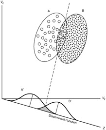
The following code displays histograms and density plots for the observations in each group on the first linear discriminant dimension. There is one panel for each group and they all appear lined up on the same graph.

# Panels of histograms and overlayed density plots
# for 1st discriminant function
plot(fit, dimen=1, type="both") # fit from lda

 click to view

The partimat( ) function in the klaR package can display the results of a linear or quadratic classifications 2 variables at a time.

# Exploratory Graph for LDA or QDA
library(klaR)
partimat(G~x1+x2+x3,data=mydata,method="lda")

 click to view

You can also produce a scatterplot matrix with color coding by group.

# Scatterplot for 3 Group Problem 
pairs(mydata[c("x1","x2","x3")], main="My Title ", pch=22, 
   bg=c("red", "yellow", "blue")[unclass(mydata$G)])

 click to view

Ref: https://www.statmethods.net/advstats/discriminant.html